Signals-Before-Stormsresearch log, in the order it happenedIndia 2016-07-22 to 2023-12-29, n = 1,814
The model worked. The strategy did not.
A Hidden Markov Model regime overlay for tactical asset allocation,
run leak-proof over eight years of Indian and US markets.
No book here separates from a static 60/40 or equal weight once the
comparison uses a paired difference test. What the overlay does buy is drawdown, cutting the
worst loss by roughly two thirds on Indian data. Published as a negative result with a
diagnosis, and it retracts one of its own findings.
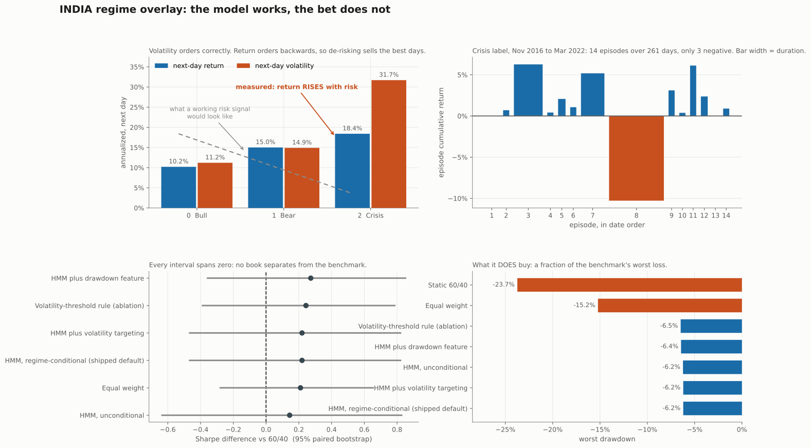
The whole argument in four panels. The states are real and persistent, but
they predict variance rather than direction (top left). The evidence behind any regime claim
is far thinner than the day count suggests (top right). No book separates from its benchmark
under a paired test (bottom left). What the overlay does buy is drawdown (bottom right).01
What was built
Three hidden states inferred from causal features, each state routed to
its own convex program. The interesting engineering is not the model, it is the two places the
pipeline refuses to look at the future.
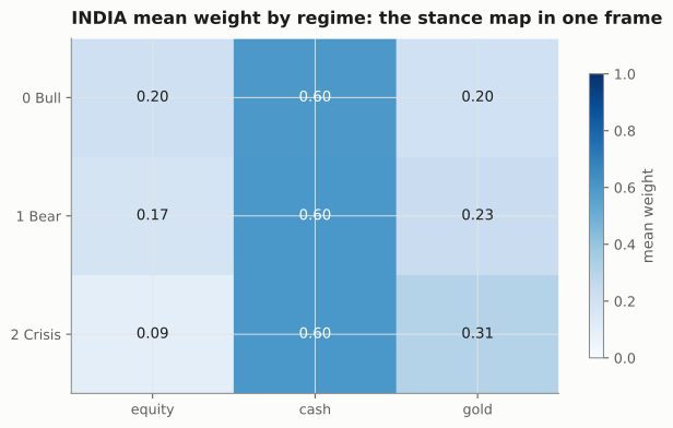
The stance map
Each regime gets a distinct convex program. Long-only,
fully invested, weight-capped.
Regime
Objective
Reasoning
0 Bull
Maximise Sharpe
Calm market, take risk
1 Bear
Minimise variance
Stressed, preserve capital
2 Crisis
Minimise variance, hard equity cap
Violent, de-risk hard
The states are not noise. The transition matrix diagonal runs 0.97 to
0.98, so the regimes persist rather than flickering. The corner entries are zero: Bull never
jumps straight to Crisis and Crisis never jumps straight to Bull, so the market always passes
through the middle state. Nothing in the fit asked for that.
Persistence, and the two corners that stay empty. Read a row: given
today's state, where tomorrow lands. The market cannot skip the middle state in either
direction, which nothing in the fit asked for.How long a state lasts, and how much of the record it owns. Crisis is
both the shortest-lived and the rarest, which is the first hint that its sample is thinner
than its day count suggests.
02
The first result, and the whole problem
Measured at the lag the strategy actually trades: the label is known at
the close of day t, the return is earned on day t plus one.
Next-day annualised return and volatility by regime
label, both universes.
Regime label
India days
India return
India vol
US days
US return
US vol
0 Bull
821
+10.2%
11.2%
665
+10.9%
8.7%
1 Bear
731
+15.0%
14.9%
841
+14.7%
15.6%
2 Crisis
261
+18.4%
31.7%
379
+16.1%
32.2%
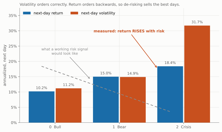
Volatility orders perfectly with the label. Return orders backwards, on both
universes. That single table explains the entire result. De-risking on the Crisis
label means selling the highest-returning days, because the rebounds of April 2020 and late
2022 are as violent as the crashes that preceded them.
A state variable has to predict direction before a directional bet on it can pay.
Realised volatility is symmetric in sign by construction, so it cannot tell a crash from a
rebound. The model was asked for regimes and it delivered regimes. They are the wrong kind.
The measured slope beside the expected one. The volatility bars climb the
way a risk-ordered label should. The return bars climb too, which is exactly backwards from
what the stance map is betting on.03
Four rescues, each judged against a criterion written down first
The obvious response to a broken result is to fix it. Every attempt was
given a success criterion before it was run, so that the outcome could not be reinterpreted
afterwards.
Re-rank the states by return
Criterion: a return-ranked ordering should separate direction where a volatility-ranked one does not.
criterion not metUS Sharpe moved 0.542 to 0.620, still under 60/40, and the crisis label came out
identical: the same 379 days at the same +16.1%. Reordering cannot add information the state space does not contain.
A structurally different estimator
Criterion: a Statistical Jump Model should find a different partition, and a directional one.
criterion not metIt does find a different partition, agreeing with the HMM only 57.5% of the time on India,
and it does what it advertises: US dwell time 27 days to 194, turnover 4.19x to 1.46x. Its US crisis label still carries the
highest forward return, +20.0%. Two estimators, same broken ordering.
Volatility targeting at 10%
Criterion: if the book is taking too much risk in the wrong states, a constant risk budget should help.
criterion not metUS 0.542 to 0.562, and bit-identical on India at 0.824. It barely binds, because minimum
variance already pins the book at 9.6% volatility on the US and 3.9% on India. The strategy is not taking too much risk. It is taking far too little.
Add a drawdown feature
Criterion, written down first: the crisis label's forward return must turn negative.
criterion not metIt went the other way on both universes: US +16.1% to +17.6%, India +18.4% to
+29.7%. It also happens to top the India Sharpe table at 0.877, and it is still not counted as a win and not
adopted as the default. Promoting it on a metric other than its stated one is precisely the selection bias the pre-registration exists to prevent.
Why volatility targeting had nothing to bind on. The stance map does exactly
what it was told, and this is the cost: equity never exceeds a quarter of the book in any
regime. The overlay is not too aggressive, it is permanently defensive.04
The retraction
One result did look like a genuine directional state. It was written up.
Then it was counted properly, and withdrawn the same day.
The Jump Model's India crisis label reads -17.1% annualised over 94
days, which would have made it the only negative-return state anywhere in this project.
It is two episodes: 64 days across COVID at -10.70%, and 30 days in late 2018
at +4.41%. Excluding COVID the label runs +30.17% annualised,
the same backwards ordering as everything else.
Worse, a cross-tabulation put all 94 of those days inside the HMM's own crisis
label, so it was never a different state space to begin with. The effective sample was one
event. The finding is retracted here rather than quietly dropped.
Days are not a sample size
That retraction came out of a general check: a claim about a regime is supported by how many
times the regime occurred, not how many rows it spanned. Drop each label's single
longest episode and see what survives.
India, out-of-sample. Effective sample size and what
remains without the largest episode.
Regime label
Episodes
Annualised return
Excluding largest episode
0 Bull
27
+10.2%
+2.7%
1 Bear
30
+15.0%
+13.1%
2 Crisis
14
+18.4%
+53.6%
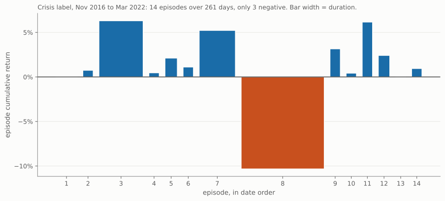
The crisis label spans 261 days, which sounds like evidence, across just 14
episodes, only 3 of which lost money. Drop the longest one and the label runs +53.6%
annualised. The backwards return ordering is not an artifact of one event: it survives episode
counting on both universes.
Fourteen episodes, not 261 days. The open dot is the label's return over
every episode; the filled dot is the same return with the single longest episode dropped.
Crisis has the fewest episodes and moves furthest, from +18.4% to +53.6%. Any claim resting
on this label rests on a sample of fourteen, and mostly on one of them.05
The comparison was wrong too
An earlier draft compared strategies by checking whether their separate
confidence intervals overlapped. That is not a comparison, and correcting it changed what could
honestly be claimed.
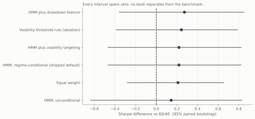
Each marginal interval asks whether one book's Sharpe differs from zero. The question that
matters is whether the gap between two books differs from zero, which needs the
interval of the difference, resampled on the same dates for both books. Since every book holds
the same assets on the same days, differencing cancels the shared market move and the paired
interval comes out roughly three times tighter.
India. Sharpe difference against each benchmark, with
its paired bootstrap interval.
Book
vs 60/40
vs equal weight
HMM plus drawdown feature
+0.273 (-0.36, +0.86)
+0.063 (-0.19, +0.28)
Volatility-threshold rule
+0.244 (-0.39, +0.79)
+0.033 (-0.23, +0.28)
HMM, regime-conditional
+0.220 (-0.47, +0.83)
+0.009 (-0.28, +0.26)
Every book, against either benchmark. The dot is the Sharpe difference and
the rule is its paired 95% interval. Every one of them crosses the zero line, which is the
claim: indistinguishable, not beaten.
Every interval spans zero, on both universes. The "it is all noise" reading
survives, and it is now earned rather than assumed. It also sharpens one claim that used to be
overstated: on the US the volatility rule's marginal interval excludes zero, which says
only that its Sharpe beats zero. Paired against 60/40 it is +0.268 (-0.029, +0.559), so even the
ablation that wins the US table cannot be said to beat the benchmarks.
06
What held up
A negative result is only worth reading if the machinery that produced
it is trustworthy. These are the checks that survived their own scrutiny.
heldLeak-proofing, asserted by tests
Lookahead bias is the easiest way to produce a beautiful, worthless backtest. Five defences,
each pinned by a unit test that fails if the defence is removed: causal right-aligned features,
standardisation fit on training rows alone, a per-fold model refit, causal forward-filter
decoding instead of whole-sequence Viterbi, and a one-day execution lag enforced in a single
shared code path so every strategy and benchmark inherits it.
heldDeflation at an honest trial count
A Sharpe reported once, from one strategy out of several tried, is a biased number. The
deflated Sharpe here charges for 7 trials, stated openly. The volatility rule
read 0.928 at 4 trials, and searching three more ideas lowered every number in that column.
That is what deflation is for. Intervals use a Politis-Romano stationary bootstrap with the
block length read off the data rather than guessed.
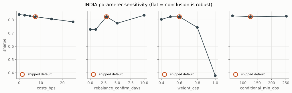
heldSensitivity reported as a surface, adopting nothing
Costs are not the story. Sharpe moves only 0.841 to 0.785 across free
trading to 25 basis points. At zero cost the strategy still does not beat its benchmarks,
which is a cleaner statement of the result than any net number.
The sweep reports the whole surface and adopts nothing, because picking the
best cell would be a search and would owe the deflated Sharpe another trial. Two knobs,
weight_cap and rebalance_confirm_days, are not flat, and the shipped
defaults sit at local Sharpe optima. Both were fixed before any result was computed and neither
is re-chosen, but a reader is entitled to be told.
heldVendor data guarded, not trusted
GOLDBEES.NS on Yahoo prints a 100x round trip over 2019-12-19 to 2019-12-23: log returns of
-4.61 then +4.61. Two bad prints in 2,193 rows. Left alone they inflate gold's return standard
deviation from 0.011 to 0.139 and poison every Indian covariance, regime fit and Sharpe. The
guard rejects any daily absolute log return above 0.5 with a loud warning, and a test pins that
a genuine -13% crash day still survives it.
heldA no-model ablation that can beat the model
The strongest control here is a two-line volatility-threshold rule: same optimiser, same
costs, same walk-forward, but the regimes come from a trailing-volatility quantile instead of
the HMM. If the HMM cannot beat that, the HMM is decoration. On the US the rule wins outright,
0.958 against 0.542.
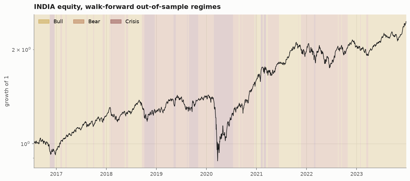
Out-of-sample labels, no future information. The causal filter independently
flags February 2018, Q4 2018, COVID and 2022. The states are real. That was never the part
that failed.07
The scorecards
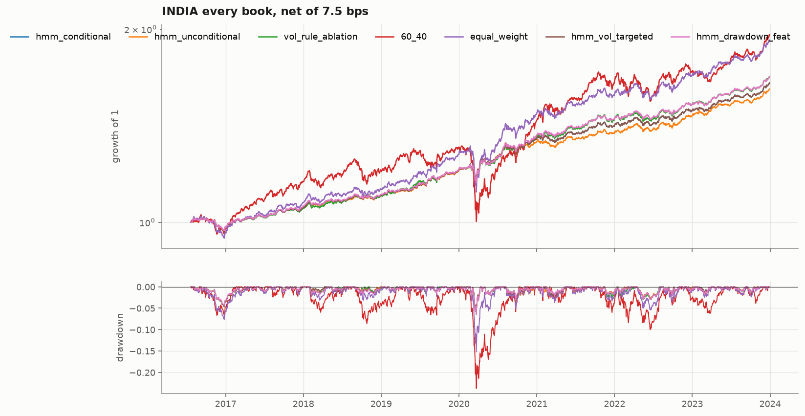
Every book, strategy and benchmark alike, runs through the same cost
engine at 7.5 basis points per unit of turnover with a one-day execution lag. A benchmark costed
on different terms is not a benchmark.
loading
India, the primary universe. Out-of-sample 2016-07-22 to
2023-12-29, n = 1,814. Sharpe is measured against the 3.79% risk-free rate the cash sleeve
actually paid, because scoring against zero would hand every defensive book a free Sharpe for
holding cash. Benchmark rows are set in italic.
Book
Sharpe (net)
Sharpe (gross)
Sortino
Max drawdown
Calmar
Turnover/yr
HMM plus drawdown feature
0.877
0.896
1.291
-6.4%
1.169
0.99x
Volatility-threshold rule (ablation)
0.848
0.863
1.244
-6.5%
1.165
0.88x
Jump Model regimes
0.829
0.833
1.204
-7.3%
1.038
0.24x
HMM, regime-conditional (shipped default)
0.824
0.841
1.211
-6.2%
1.161
0.87x
HMM plus volatility targeting
0.824
0.841
1.211
-6.2%
1.161
0.87x
Equal weight
0.815
0.819
1.167
-15.2%
0.625
0.41x
HMM, unconditional
0.748
0.758
1.097
-6.2%
1.103
0.50x
Static 60/40 (equity/cash)
0.604
0.607
0.827
-23.7%
0.413
0.36x
Read the Sharpe column and the strategy is unremarkable. The overlay's point
estimate sits above both benchmarks, and entry 05 is the reason that means nothing: no book here
is statistically distinguishable from either one. Read max drawdown and Calmar, the other
two metrics the brief names, and the picture inverts: -6.2% worst drawdown against
-15.2% and -23.7%, with Calmar roughly 1.9x and 2.8x the benchmarks. That gap is not noise, it is
the mechanical consequence of routing to minimum variance whenever the label is not calm. The
overlay buys drawdown protection and pays for it in return. Whether that trade is worth making is
a mandate question, not a statistical one.
The trade, drawn. The benchmark ends higher. The overlay never falls far.
Those are the same fact seen twice. Hover either chart and both cursors move together.
US, the robustness universe. Out-of-sample 2016-07-05 to
2023-12-29, n = 1,886, risk-free rate zero, with a real bond sleeve. Benchmark rows are set in
italic.
Book
Sharpe (net)
Max drawdown
Calmar
Turnover/yr
Volatility-threshold rule (ablation)
0.958
-21.9%
0.446
3.61x
Static 60/40
0.690
-27.6%
0.273
0.41x
Jump Model regimes
0.682
-25.1%
0.262
1.46x
Equal weight
0.650
-23.0%
0.258
0.42x
HMM plus drawdown feature
0.590
-28.0%
0.191
3.88x
HMM plus volatility targeting
0.562
-27.3%
0.182
4.10x
HMM, regime-conditional
0.542
-28.7%
0.170
4.19x
HMM, unconditional
0.535
-27.4%
0.174
2.74x
The US does not reproduce India, and saying so is the point of running it.
No HMM book improves on either benchmark on Sharpe or Calmar, and the drawdown protection that
vindicated the overlay on India does not reappear: the best HMM drawdown here is level with
60/40 and well behind equal weight at -23.0%. Minimum variance had nowhere to hide in 2022, when
bonds fell alongside equities. A result that held on one market and was quietly assumed to hold on the
other would be the more comfortable story. It is not the one the data tells.
One more thing the sweep decided rather than assumed. Three regimes were
chosen to match the economic states being allocated against, then checked with a BIC sweep. It
supports three on the primary Indian universe, where the step from three states to four buys
only 392 of fit against 6,256 for the step from two to three. It does not support three on the
US. Both are reported.
08
The verdict
Hidden Markov states on returns and volatility are volatility states, and
volatility carries no directional information. That is the finding, and it outlives this
codebase.
Realised volatility and VIX are symmetric in sign by construction. Any allocator built on
them alone will de-risk into rebounds as reliably as into crashes, because it cannot tell the
two apart. Finding a directional state needs a signed state variable: credit spreads, market
breadth, earnings revisions, positioning, realised skew. Not another estimator on the same
features.
The one thing the overlay does buy is drawdown, and only on one of the two universes tested.
Two of the three metrics the brief names favour it there. That is reported as exactly what it
is, on one universe, rather than promoted into a headline.